
|
|
|
| |
|
|
|
|
|
Differential EquationsIn physics we come across a variety of problems which require the use of Differential Equations in order to solve. We'll start with a simple example and then expand upon it gradually. For instance, how would you mathematically model the motion of a spring or a pendulum where the forces are constantly changing at every point?
Solution MethodsThe solutions to differential equations are what physicists are most interested in, since it's the solutions which dictate the allowable types of behavior for the system and not the differential equation itself.
There are a variety of methods which can be used for solving various forms of Differential Equations. 1. First identify the form of the differential equation, or perform algebra to convert an equation (or set of equations) into a recognizable differential equation form. Usually you want to try forms that are easiest to solve first. 2. Second is to use the appropriate solution method, sometimes these methods will not work and you will need to use other methods such as "Special Integrating Factors" or a "Variation of Parameters". 3. Third and last is "Plug It In!", Check and see if your derived solution actually satisfies the differential equation. If it doesn't work, go back to step 2 and try another solution method. Linear EquationsThe easiest solution method is known as "Separation of Variables", where (as the name implies) you literally separate the variables using algebra and then use calculus to integrate both sides and the result is your solution. Generally this method works best for Linear Equations with two variables, which are then separated to opposite sides of the equals sign.
Take, for example, the force "F" of a spring with spring constant "k"; F=-kx
We also know that force equals mass x acceleration (Newton's 2nd Law) F=ma dx = space differential ; dt = time differential
In terms of differentials our equations looks more like -kx = m * d2x/dt2 The next step is to get all the t's and dt's (time-like stuff) on one side of the equation and all the x's and dx's (space-like stuff) onto the other side. This is called "Separation of Variables" for a good reason. So we just multiply both sides by dt2 and divide both sides by x and we get; -kdt2x/x = mdx/x On the left side we have x/x which is just equal to 1 since anything divided by itself is just =1, so this disappears. We are tempted to do the same on the right side of the equation "mdx/x" except that the x on top is dx not x which is different, so we must be careful. dx/x is actually 1/x*dx . In any case our equation is now -kdt2 = 1/x*mdx , which is separated and now solvable by integral calculus. The integral of 1/x gives us a logarithm "log(x)" which you can then get rid of if you raise both sides of the equation as e to the power of. I won't go into all the steps in between, for those I suggest you review the Calculus and Algebra sections. The solution ends up being: x = esqrt(k/m) * t ; which is just the 1D equation for a wave x=ewt , where w=sqrt(k/m) is the angular frequency of oscillation, which can easily be converted to the actual frequency by a factor of 2pi. This factor is there any time you have e^ to the power of something. Even though separation of variables requires the knowledge and application of a variety of algebra and calculus operations, it is actually one of the easiest methods for solving differential equations. But it turns out that you needn't go through all these steps every single time. By knowing the form these equations take and how that effects the form of the solution, we can use short-cuts to "guess" solutions which we assume will work, then test them to see if, indeed, they do work. Exact EquationsExact equations are also generally easy to recognize and solve. If you see an equation that looks like the form: Pdx + Qdy = 0 ; Where P and Q are both functions of x and/or y To tell if an equation is exact, you just look at the opposing derivatives of P and Q. Since P is with dx you will want to take the derivate with respect to y, and since Q is with dy you will want to take the derivate of Q with respect to x. So just look at the functions P and Q in front of dx and dy and take the derivate of P and Q with respect to the opposite variables, and check to see if they are equal. If they are equal then the equation is exact and you can go on to use the Exact Equation Solution Method below. If they aren't equal, then the equation isn't exact and you will have to try a different solution method. Exact Equation Solution MethodFinding a solution to an exact differential equation is pretty straight-forward, the first step is to integrate Pdx, and Qdy. Once you find the indefinite integral of both of these, you look at the terms from each that are similar and find the terms that are different. The similar terms do not need to be repeated. Basically just pick one of the equations and add the different terms from the other equation onto your first equation, and that total of all these terms together should give you your solution. The idea is that the different terms will have respective (x and y) derivatives which go to zero on each side to leave you with P and Q. So that when you take the derivatives of your determined solution with respect to x and y, you end up with P and Q respectively. Examples and a Table of different formulas coming soon.
---------User feedback and interest in this area will determine how much work I put into this section------
Homogeneous EquationsSpecial Integrating FactorsBernoulli EquationNon-Homogeneous EquationsUndetermined Coefficients MethodVariation of Parameters MethodWronskiansNon-Linear Diff. Eq'sImportant Physics Applications of Diff EqsRLC Circuits
In this circuit, the three components are all in series with the voltage source. The governing differential equation can be found by substituting into Kirchhoff's voltage law (KVL) the constitutive equation for each of the three elements. From KVL, where For the case where the source is an unchanging voltage, differentiating and dividing by L leads to the second order differential equation: This can usefully be expressed in a more generally applicable form:
For the case of the series RLC circuit these two parameters are given by:[3]
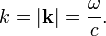
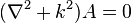
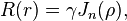
A useful parameter is the damping factor, ? which is defined as the ratio of these two, In the case of the series RLC circuit, the damping factor is given by, The value of the damping factor determines the type of transient that the circuit will exhibit.[4] Some authors do not use The Helmholtz EquationThe Helmholtz equation, named for Hermann von Helmholtz, is the elliptic partial differential equation where ?2 is the Laplacian, k is the wavenumber, and A is the amplitude.
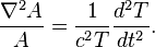
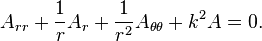
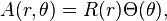
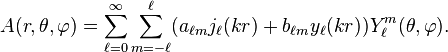
Motivation and usesThe Helmholtz equation often arises in the study of physical problems involving partial differential equations (PDEs) in both space and time. The Helmholtz equation, which represents the time-independent form of the original equation, results from applying the technique of separation of variables to reduce the complexity of the analysis. For example, consider the wave equation Separation of variables begins by assuming that the wave function u(r, t) is in fact separable: Substituting this form into the wave equation, and then simplifying, we obtain the following equation: Notice the expression on the left-hand side depends only on r, whereas the right-hand expression depends only on t. As a result, this equation is valid in the general case if and only if both sides of the equation are equal to a constant value. From this observation, we obtain two equations, one for A(r), the other for T(t): and where we have chosen, without loss of generality, the expression -k2 for the value of the constant. (It is equally valid to use any constant k as the separation constant; -k2 is chosen only for convenience in the resulting solutions.) Rearranging the first equation, we obtain the Helmholtz equation: Likewise, after making the substitution the second equation becomes where k is the wave vector and ? is the angular frequency. Harmonic solutionsIt is relatively easy to show that solutions to the Helmholtz equation will take the form: which corresponds to the time-harmonic solution for arbitrary (complex-valued) constants C and D, which will depend on the initial conditions and boundary conditions, and subject to the dispersion relation We now have Helmholtz's equation for the spatial variable r and a second-order ordinary differential equation in time. The solution in time will be a linear combination of sine and cosine functions, with angular frequency of ?, while the form of the solution in space will depend on the boundary conditions. Alternatively, integral transforms, such as the Laplace or Fourier transform, are often used to transform a hyperbolic PDE into a form of the Helmholtz equation. Because of its relationship to the wave equation, the Helmholtz equation arises in problems in such areas of physics as the study of electromagnetic radiation, seismology, and acoustics. Solving the Helmholtz equation using separation of variablesThe general solution to the spatial Helmholtz equation can be obtained using separation of variables. Vibrating membraneThe two-dimensional analogue of the vibrating string is the vibrating membrane, with the edges clamped to be motionless. The Helmholtz equation was solved for many basic shapes in the 19th century: the rectangular membrane by Siméon Denis Poisson in 1829, the equilateral triangle by Gabriel Lamé in 1852, and the circular membrane by Alfred Clebsch in 1862. The elliptical drumhead was studied by Émile Mathieu, leading to Mathieu's differential equation. The solvable shapes all correspond to shapes whose dynamical billiard table is integrable, that is, not chaotic. When the motion on a correspondingly-shaped billiard table is chaotic, then no closed form solutions to the Helmholtz equation are known. The study of such systems is known as quantum chaos, as the Helmholtz equation and similar equations occur in quantum mechanics. If the edges of a shape are straight line segments, then a solution is integrable or knowable in closed-form only if it is expressible as a finite linear combination of plane waves that satisfy the boundary conditions (zero at the boundary, i.e., membrane clamped). An interesting situation happens with a shape where about half of the solutions are integrable, but the remainder are not. A simple shape where this happens is with the regular hexagon. If the wavepacket describing a quantum billiard ball is made up of only the closed-form solutions, its motion will not be chaotic, but if any amount of non-closed-form solutions are included, the quantum billiard motion becomes chaotic. Another simple shape where this happens is with an "L" shape made by reflecting a square down, then to the right. If the domain is a circle of radius a, then it is appropriate to introduce polar coordinates r and ?. The Helmholtz equation takes the form We may impose the boundary condition that A vanish if r=a; thus The method of separation of variables leads to trial solutions of the form where T must be periodic of period 2p. This leads to and It follows from the periodicity condition that and that n must be an integer. The radial component R has the form where the Bessel function Jn(?) satisfies Bessel's equation
and ?=kr. The radial function Jn has infinitely many roots for each value of n, denoted by ?m,n. The boundary condition that A vanishes where r=a will be satisfied if the corresponding wavenumbers are given by The general solution A then takes the form of a doubly infinite sum of terms involving products of These solutions are the modes of vibration of a circular drumhead. Three-dimensional solutionsIn spherical coordinates, the solution is: This solution arises from the spatial solution of the wave equation and diffusion equation. Here are the spherical harmonics (Abramowitz and Stegun, 1964). Note that these forms are general solutions, and require boundary conditions to be specified to be used in any specific case. For infinite exterior domains, a radiation condition may also be required (Sommerfeld, 1949). For where function is called scattering amplitude and u0(r0) is the value of A at each boundary point r0. Paraxial approximationThe paraxial approximation of the Helmholtz equation is: where This equation has important applications in the science of optics, where it provides solutions that describe the propagation of electromagnetic waves (light) in the form of either paraboloidal waves or Gaussian beams. Most lasers emit beams that take this form. In the paraxial approximation, the complex magnitude of the electric field E becomes where A represents the complex-valued amplitude of the electric field, which modulates the sinusoidal plane wave represented by the exponential factor. The paraxial approximation places certain upper limits on the variation of the amplitude function A with respect to longitudinal distance z. Specifically: and These conditions are equivalent to saying that the angle ? between the wave vector k and the optical axis z must be small enough so that The paraxial form of the Helmholtz equation is found by substituting the above-stated complex magnitude of the electric field into the general form of the Helmholtz equation as follows. Expansion and cancellation yields the following: Because of the paraxial inequalities stated above, the ?2A/?z2 factor is neglected in comparison with the ?A/?z factor. The yields the Paraxial Helmholtz equation. Inhomogeneous Helmholtz equationThe inhomogeneous Helmholtz equation is the equation where : Rn ? C is a given function with compact support, and n = 1, 2, 3. This equation is very similar to the screened Poisson equation, and would be identical if the plus sign (in front of the k term) is switched to a minus sign. In order to solve this equation uniquely, one needs to specify a boundary condition at infinity, which is typically the Sommerfeld radiation condition uniformly in With this condition, the solution to the inhomogeneous Helmholtz equation is the convolution (notice this integral is actually over a finite region, since f has compact support). Here, G is the Green's function of this equation, that is, the solution to the inhomogeneous Helmholtz equation with equaling the Dirac delta function, so G satisfies The expression for the Green's function depends on the dimension n of the space. One has for n = 1, for n = 2, where for n = 3. Note that we have chosen the boundary condition that the Green's function is an outgoing wave for References
External links
|


 are the voltages across R, L and C respectively and
  is the time varying voltage from the source. Substituting in the constitutive equations,
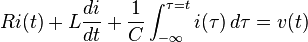


 and
and  are both in units of
  and
and 


 and call
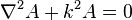


 and
and  are the
 function

 is the transverse part of the


 with
with  , where the vertical bars denote the
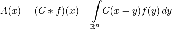


 is a
is a 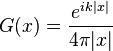
 .
.